7.15 kmeans example wine normalised cluster
20211231
The different variables of the wine dataset have quite different scales and so normalisation is appropriate to better suit the distance calculations used by k-means discussed in Section 7.13.
As a pipeline, we normalise the data,
tee it to norm.csv, train
3 clusters, predict and save the clusters as
the column label in the file wine.pr using mlr:
cat wine.csv |
  ml normalise kmeans |
  tee norm.csv |
  ml train kmeans 3 |
  ml predict kmeans norm.csv |
  mlr --csv cut -f label > wine.pr
These predictions of cluster membership are then compared to the
original wine.data file class, though noting that a cluster
analysis is not a supervised classification task as such. We
cat the original data file, cut
the first field, use awk to add a column name of
class as the header, paste the class to the
predictions from wine.pr, remove the header by taking the
tail from line 2, sorting the
resulting rows and counting the number of unique
rows:
cat wine.data |
  cut -d"," -f 1 |
  awk 'NR ==1{ print "class "} {print}' |
  paste -d"," - wine.pr |
  tail +2 |
  sort |
  uniq -c
Now cluster 0 predominately matches class 1, cluster 2 class 2 and cluster 1 class 3:
59 1,0
10 2,0
9 2,1
52 2,2
2 3,0
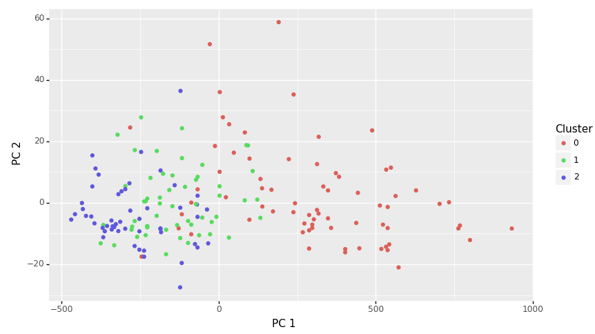
46 3,1The plot is interestingly more dispersed (c.f. Section 7.14. See Section 7.16 for an explanation.
Your donation will support ongoing availability and give you access to the PDF version of this book. Desktop Survival Guides include Data Science, GNU/Linux, and MLHub. Books available on Amazon include Data Mining with Rattle and Essentials of Data Science. Popular open source software includes rattle, wajig, and mlhub. Hosted by Togaware, a pioneer of free and open source software since 1984. Copyright © 1995-2022 Graham.Williams@togaware.com Creative Commons Attribution-ShareAlike 4.0